deconvoluting_spatial_data_with_panpipes.md

Deconvoluting spatial data with Panpipes

The deconvolution_spatial workflow runs deconvolution for spatial data. Multiple slides can be deconvoluted with the same reference in one run. For each spatial slide, the workflow expects one MuData object, with the spatial data saved in mudata.mod['spatial']. For the reference scRNA-Seq data, it expects a MuData, with the gene expression data saved in mudata.mod['rna']. The steps of the workflow are explained in greater detail here.

For all the tutorials, we will append the --local command which ensures that the pipeline runs on the computing node you're currently on, namely your local machine or an interactive session on a computing node on a cluster.

Directories and data

For the deconvolution tutorial, we will work in the main directory spatial and create a deconvolution directory for the deconvolution:

# mkdir spatial # <- if you don't have the spatial directory already 
# cd spatial
mkdir deconvolution deconvolution/data deconvolution/data/spatial_data
cd deconvolution

In this tutorial, we will use human heart spatial transcriptomics and scRNA-Seq data published by Kuppe et al. You can use the following python code to download and save the data as MuData files:

import scanpy as sc
import muon as mu

# Loading the spatial data: 
adata_st = sc.read(
    filename="kuppe_visium_human_heart_2022_control.h5ad",
    backup_url="https://figshare.com/ndownloader/files/39347357",
)
# In this tutorial, we will only use the spatial slide of patient 'P1'
adata_st = adata_st[adata_st.obs["patient"] == "P1"]
del adata_st.uns["spatial"]["control_P17"]
del adata_st.uns["spatial"]["control_P7"]
del adata_st.uns["spatial"]["control_P8"]
mu.MuData({"spatial": adata_st}).write_h5mu("./data/spatial_data/Human_Heart.h5mu")

# Loading the single-cell reference
adata_sc = sc.read(
    filename="kuppe_snRNA_human_heart_2022_control.h5ad",
    backup_url="https://figshare.com/ndownloader/files/39347573",
)
adata_sc.X = adata_sc.layers["counts"]
adata_sc.var.index = adata_sc.var["feature_name"]
mu.MuData({"rna": adata_sc}).write_h5mu("./data/Human_Heart_reference.h5mu")

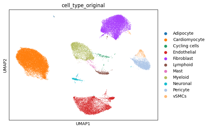
The spatial slide and single-cell reference data we will be using looks as follows:

The structure of the deconvolution directory after downloading the data:

deconvolution
└──  data
	|── Human_Heart_reference.h5mu
	└──  spatial_data
		└── Human_Heart.h5mu

Note, that the MuData object of the reference data should not be saved into the same folder as the spatial data! When running the workflow, the workflow expects all spatial MuData objects to be saved in the same folder and reads in all MuData objects of that directory. When saving the reference MuData into the same folder as the spatial, the workflow would treat the reference MuData as spatial and would try to run deconvolution on it.

Cell2Location

Edit yaml file

In spatial/deconvolution, create the pipeline.yml and pipeline.log files by running panpipes deconvolution_spatial config in the command line (you potentially need to activate the conda environment with conda activate pipeline_env first!). Modify the yaml file, or simply use the pipeline.yml that we provide (you potentially need to add the path of the conda environment in the yaml).

Run Panpipes

Run the full workflow with panpipes deconvolution_spatial make full --local.

Once Panpipes has finished, the spatial/deconvolution directory will have the following structure:

deconvolution
├── cell2location.output
│   └── Human_Heart
│		├── Cell2Loc_inf_aver.csv
│		├── Cell2Loc_screference_output.h5mu
│		└── Cell2Loc_spatial_output.h5mu
├── data
│	|── Human_Heart_reference.h5mu
│	└──  spatial_data
│		└── Human_Heart.h5mu
├── figures
│   └── Cell2Location
│   	└── Human_Heart
│       	├── ELBO_reference_model.png
│       	├── ELBO_spatial_model.png
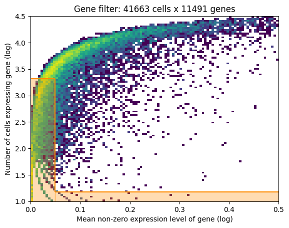
│       	├── gene_filter.png
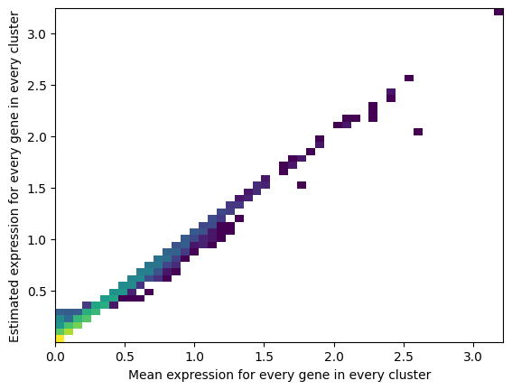
│       	├── QC_reference_expression signatures_vs_avg_expression.png
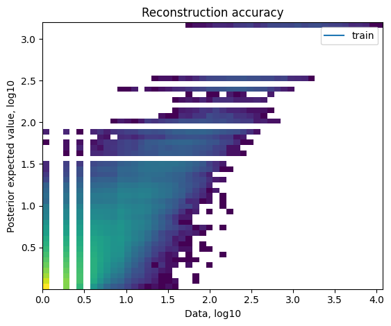
│       	├── QC_reference_reconstruction_accuracy.png
│       	├── QC_spatial_reconstruction_accuracy.png
│       	└── show_Cell2Loc_q05_cell_abundance_w_sf.png
├── logs
│   └── Cell2Location_Human_Heart.log
├── pipeline.log
└── pipeline.yml

In the folder ./cell2location.output a folder for each slide will be created containing the following outputs:

• MuData containing the spatial data together with the posterior of the spatial mapping model
• MuData containing the reference data together with the posterior of the reference model
• A csv-file Cell2Loc_inf_anver.csv containing the estimated expression of every gene in every cell type
• If save_models = True, the reference model and the spatial mapping model

Also in ./figures/Cell2Location, a folder for each slide will be created. Each folder will contain the following plots:

• If gene selection according to Cell2Location is performed: a plot of the gene filtering

• For both models:
  • QC plots

• ELBO plots
• Spatial plot where the spots of the slide are colored by the estimated cell type abundances

Note: We find that keeping the suggested directory structure (one main directory by project with all the individual steps in separate folders) is useful for project management. You can of course customize your directories as you prefer, and change the paths accordingly in the pipeline.yml config files!