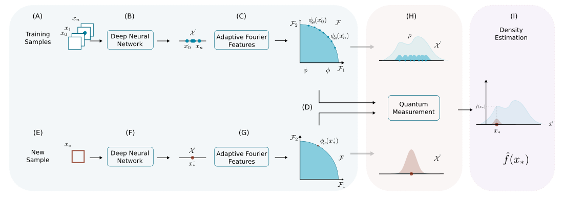
DEMANDE: Density Matrix Neural Density Estimation

DEMANDE (Density Matrix NEural Density Estimation) is a neural density estimation method based on density matrices and adaptive Fourier features. It provides a flexible machine-learning approach to estimate probability density functions from data, grounded in the mathematical formalism of density matrices commonly used in quantum mechanics. (IEEE)

---

📌 Overview

Traditional density estimation methods like Kernel Density Estimation (KDE) scale poorly with dimensionality and dataset size. DEMANDE models densities using density matrices combined with adaptive Fourier feature maps, yielding a scalable, data-driven estimator that can be integrated with deep learning tools and evaluated efficiently. (IEEE)

---

🔍 Features

• Density matrix representation of probability distributions
• Adaptive Fourier features to approximate kernels and embed data
• Python implementation with example notebooks
• Modular and extensible for research and experiments
• Includes tests and baseline usage examples

---

🚀 Getting Started

Setup

Installation

Install Miniconda from here and then run the following commands to create the demande environment:

conda env create -f environment.yml

conda activate demande

Next, install the package:

pip install -e .

or if you want development dependencies as well:

pip install -e .[dev]

Create Directories

• mkdir reports mlflow data

Ml-flow

All the experiments will be saved on Ml-flow in the following path using sqlite: mlflow/

mkdir mlflow/

After running your experiments, you can launch the ml-flow dashboard by running the following command:

mlflow ui --port 8080 --backend-store-uri sqlite:///mlflow/tracking.db

Dataset

The dataset is publicly available in Zenodo

The dataset contains the features and probabilities of ten different functions.
Each dataset is saved using NumPy arrays.

Arc

The dataset Arc corresponds to a two-dimensional random sample drawn from a random vector

$$ X = (X_1, X_2) $$

with probability density function

$$ f(x_1, x_2) = \mathcal{N}(x_2 \mid 0, 4); \mathcal{N}(x_1 \mid 0.25x_2^2, 1) $$

where $\mathcal{N}(u \mid \mu, \sigma^2)$ denotes the density function of a normal distribution with mean $\mu$ and variance $\sigma^2$.

:contentReference[oaicite:0]{index=0} used this dataset to evaluate neural density estimation methods (2017).

---

Potential 1

The dataset Potential 1 corresponds to a two-dimensional random sample drawn from a random vector

$$ X = (X_1, X_2) $$

with probability density function

$$f(x_1, x_2) = \frac{1}{2}\left(\frac{\|x\|-2}{0.4}\right)^2 - \ln\left( \exp\left\{-\frac{1}{2}\left(\frac{x_1-2}{0.6}\right)^2\right\} + \exp\left\{-\frac{1}{2}\left(\frac{x_1+2}{0.6}\right)^2\right\} \right)$$

The normalizing constant is approximately 6.52, calculated using Monte Carlo integration.

---

Potential 2

The dataset Potential 2 corresponds to a two-dimensional random sample drawn from a random vector

$$ X = (X_1, X_2) $$

with probability density function

$$ f(x_1, x_2) = \frac{1}{2}[ \frac{x_2 - w_1(x)}{0.4} ]^2 $$

where

$$ w_1(x) = \sin(\frac{2\pi x_1}{4}) $$

The normalizing constant is approximately 8, calculated using Monte Carlo integration.

---

Potential 3

The dataset Potential 3 corresponds to a two-dimensional random sample drawn from a random vector

$$ X = (X_1, X_2) $$

with probability density function

$$f(x_1, x_2) = - \ln( \exp\{-\frac{1}{2}[\frac{x_2-w_1(x)}{0.35}]^2\} + \exp\{-\frac{1}{2}[\frac{x_2-w_1(x)+w_2(x)}{0.35}]^2\} )$$

where

$$ w_1(x) = \sin(\frac{2\pi x_1}{4}) $$

and

$$ w_2(x) = 3 \exp{ -\frac{1}{2} [\frac{x_1-1}{0.6}]^2 } $$

The normalizing constant is approximately 13.9, calculated using Monte Carlo integration.

---

Potential 4

The dataset Potential 4 corresponds to a two-dimensional random sample drawn from a random vector

$$ X = (X_1, X_2) $$

with probability density function

$$f(x_1, x_2) = - \ln( \exp\{-\frac{1}{2}[\frac{x_2-w_1(x)}{0.4}]^2\} + \exp\{-\frac{1}{2}[\frac{x_2-w_1(x)+w_3(x)}{0.35}]^2\} )$$

where

$$ w_1(x) = \sin(\frac{2\pi x_1}{4}) $$

$$ w_3(x) = 3,\sigma( [\frac{x_1-1}{0.3}]^2 ) $$

and

$$ \sigma(x) = \frac{1}{1+\exp(x)} $$

The normalizing constant is approximately 13.9, calculated using Monte Carlo integration.

---

2D Mixture

The dataset 2D mixture corresponds to a two-dimensional random sample drawn from

$$ X = (X_1, X_2) $$

with probability density

$$ f(x) = \frac{1}{2}\mathcal{N}(x \mid \mu_1, \Sigma_1) + \frac{1}{2}\mathcal{N}(x \mid \mu_2, \Sigma_2) $$

where

$$ \mu_1 = [1,-1]^T, \quad \mu_2 = [-2,2]^T $$

and

$$ \Sigma_1 = \begin{bmatrix} 1 & 0 \\ 0 & 2 \end{bmatrix}, \quad \Sigma_2 = \begin{bmatrix} 2 & 0 \\ 0 & 1 \end{bmatrix} $$

---

10D Mixture

The dataset 10D-mixture corresponds to a 10-dimensional random sample drawn from

$$ X = (X_1, \ldots, X_{10}) $$

with a mixture of four diagonal normal probability density functions

$$ \mathcal{N}(X_i \mid \mu_i, \sigma_i) $$

where

• each $\mu_i$ is drawn uniformly from the interval $[-0.5, 0.5]$
• each $\sigma_i$ is drawn uniformly from the interval $[-0.01, 0.5]$

Each component of the mixture is selected with probability

$$ \frac{1}{4} $$

---

📁 Repository Structure

📦 demande
├── src/                    # Core implementation
├──── configs/
├──── dataset_utils/
│     ├── generators/
│     ├── probability_estimators/
├──── mlflow_utils/
├──── models/
│     ├── demande/
│     └── normalizing_flows/
├──── training/
│     ├── model_building/
├──── utils/
├──── visualizations/
├── notebooks/             # Python scripts to run demos
├── tests/                  # Unit and integration tests
├── data/                   # Example dataset
├── pyproject.toml
├── environment.yaml
├── README.md
└── LICENSE

---

🧪 Testing

Run the test suite:

pytest tests/

---

📚 Related Work

DEMANDE builds on the idea of density matrices as probability density estimators, with roots in kernel and random Fourier feature methods. ([Fast Kernel Density Estimation][https://link.springer.com/chapter/10.1007/978-3-031-22419-5_14])

---

📄 Citation

If you use the ideas of this code in your research, please cite:

@article{gallego2023demande,
  title={DEMANDE: Density Matrix Neural Density Estimation},
  author={Gallego-Meji{\'a}, Joseph A. and Gonz{\'a}lez, Fabio A.},
  journal={IEEE Access},
  year={2023}
}

If you use this code in your research, please cite:

@article{gallego2023demandedataset,
  title={Demande dataset},
  author={Gallego-Mejia, Joseph A and Gonzalez, Fabio A},
  year={2023},
  publisher={Zenodo}
}

🧑‍🔬 Contributing

Contributions are welcome! Please open issues for bugs, feature requests, or improvements.

1. Fork the repo
2. Create a feature branch
3. Add tests for new behavior
4. Submit a pull request

---

📜 License

This project is licensed under the MIT License.

---

Related Work

[1]: Gallego-Mejia, J. A., & González, F. A. (2023). Demande: Density matrix neural density estimation. IEEE access, 11, 53062-53078.